Market Size Estimation for Data Center Capacity
Learn practical market size estimation methods for data center capacity and pipeline analysis, with templates, examples, and confidence ranges you can apply
17 min read
Market size estimation often gets presented as a clean number. It isn't. It's a model built from scope choices, unit choices, and assumption choices. That point matters more in digital infrastructure than in most sectors because capacity can be measured in revenue, sites, halls, cabinets, or power, and each lens produces a different answer.
The most useful starting point is blunt: market size estimation is a constructed exercise, not a directly observed fact. A practical guide to sizing markets describes the standard pattern clearly. Analysts define scope, choose top-down or bottom-up methods, often multiply potential customers by average annual revenue per customer, then validate the result with a second method and scenario ranges market sizing methodology overview. For data centers, that same logic applies, but the unit that usually matters most is not customers or revenue. It's deliverable IT capacity.
Table of Contents
- Why Data Center Capacity Makes Market Sizing Harder
- Defining Market Size Estimation and the TAM SAM SOM Stack
- Top-Down Versus Bottom-Up Methods in Practice
- Building a Bottom-Up Capacity and Pipeline Model
- Layering Top-Down Anchors and Scenario Ranges
- Turning Mixed Inputs Into Defensible Confidence Bands
- Common Pitfalls in Data Center Market Sizing
- A Practical Playbook for Your Next Estimate
Why Data Center Capacity Makes Market Sizing Harder
A software market can often be sized from customer counts and contract value. A data center market usually can't. The analyst is trying to answer a more physical question: how much capacity exists, how much is likely to come online, and how much of that capacity is relevant to the target segment.
Capacity is not one thing
A developer may report a campus in megawatts. An operator may talk about raised floor area. An investor memo may shift to revenue. A local planning file may only mention building phases and utility works. Those are all useful inputs, but they aren't interchangeable.
That mismatch creates the first distortion. A market framed as “all facilities in a region” is different from one framed as “wholesale-ready IT load.” A second distortion follows immediately. Some records describe facility load, while others point more directly to IT load. If that distinction isn't standardized before aggregation, the final market figure inherits hidden inconsistency.
Practical rule: If the estimate is meant to represent capacity supply, the model should anchor on IT load in MW and push all other units into supporting fields.
A second complication is confidence. Some site values are operator-disclosed. Others are estimated from facility attributes, deployment patterns, and known phase design. Both have value. They do not deserve the same weight.
That's why teams building operational workflows around Agentic AI data center solutions often focus less on generating a single answer and more on exposing what is known, what is inferred, and what still needs review. In capacity market sizing, the quality signal is not the neatness of the total. It's the transparency of the build.
Pipeline changes the answer before the math starts
Pipeline visibility makes the challenge harder again. A market estimate built from operational assets answers one question. A market estimate that includes under-construction and planned sites answers another. If prospective campuses are included as if they were contracted supply, the model stops being descriptive and starts becoming aspirational.
Four recurring issues usually drive the spread between one analyst's answer and another's:
- Unit drift: one part of the model uses MW, another switches to revenue or site count.
- Load ambiguity: reported capacity may reflect different load definitions across filings and operator materials.
- Confidence mismatch: disclosed MW and AI-estimated MW get blended without labeling the split.
- Stage inflation: announced, planned, under-construction, and operational capacity get treated as equally real.
Those are not edge cases. They are the core reason market size estimation in data centers requires more discipline than the textbook version suggests.
Defining Market Size Estimation and the TAM SAM SOM Stack
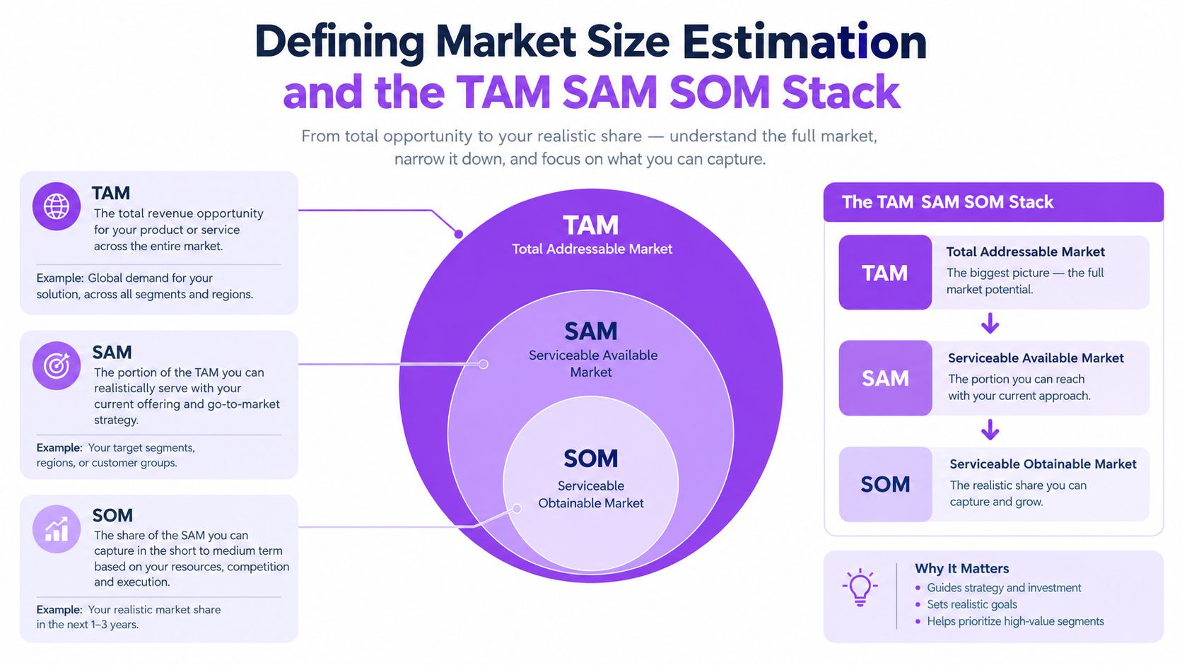
Most executives use TAM, SAM, and SOM as if they were facts waiting to be found. In practice, they're nested models. The World Bank guide on market sizing notes that credible estimates have long been grounded in public datasets such as government statistics, central banks, and trade associations, and related research shows that market potential estimation has deep roots in formal quantitative methods rather than pitch-deck shorthand historical and institutional grounding for market sizing.
What the stack means in capacity terms
In a data center context, TAM is the broadest addressable capacity universe the analyst chooses to include. That could mean global capacity across hyperscale, colocation, edge, and enterprise environments.
SAM narrows the field. It might isolate one geography, one product type, or one service standard. For example, an estimate could narrow from all addressable capacity to facilities that match a specific market segment and service profile in a selected region. Readers evaluating operator footprints often use structured directories such as data center operators by market to define that narrower universe before any math begins.
SOM is the portion that a specific operator, developer, or investment thesis could realistically capture. In digital infrastructure, that usually depends less on “demand potential” in the abstract and more on constraints such as land control, utility timing, customer mix, design standard, and permitting probability.
Why the unit changes the headline
A key point from general market sizing practice is that the selected unit materially changes the estimate. Markets can be measured by customers, companies, revenue, units, transactions, or subscriptions, and different units produce different results in the same market practical framing of market units and assumptions. In data centers, the equivalent choice is MW versus revenue versus site count versus white space.
A site-count TAM can look large while masking that many sites are small. A revenue TAM can look impressive while obscuring whether the market is constrained by available power. A capacity TAM forces the estimate back onto the infrastructure variable that determines what can be deployed.
A simple worked example
Assume an analyst starts with a 10,000 MW capacity universe for a broad region and product family.
- TAM: all 10,000 MW in the defined universe
- SAM: a narrower subset after filtering for geography, facility type, or service profile
- SOM: the realistically capturable share after applying execution constraints
The exact SAM and SOM values depend on the model's inclusion rules. That's the point. The stack isn't useful because it labels three buckets. It's useful because it forces the analyst to write down why each bucket shrinks.
Top-Down Versus Bottom-Up Methods in Practice
Top-down and bottom-up methods often get described as stylistic preferences. In capacity analysis, they are better understood as two different error profiles.
What top-down gets right
Top-down estimation starts with macro anchors, then narrows. The anchors might be operator disclosures, official statistics, trade association materials, supply-side aggregation, or other public datasets. That approach is historically standard in market sizing and remains valuable when analysts need a quick directional estimate grounded in recognized data categories.
Top-down work is efficient because it gives senior stakeholders a fast answer. It's also useful when site-level data is thin, fragmented, or delayed.
Its weakness is compression. The method tends to smooth over the differences between one facility and another, one campus phase and another, and one pipeline stage and another. In a capacity market, those differences are often where risk lives.
What bottom-up exposes
Bottom-up estimation starts from the asset list. The analyst defines the universe of facilities, standardizes the unit, classifies status, and aggregates capacity row by row. For digital infrastructure, this is usually the more defensible spine because it reveals concentration, development timing, and the split between disclosed and inferred capacity.
It is slower. That's a feature, not a flaw. The extra work forces visibility into assumptions that a top-down model can hide.
| Dimension | Top-Down | Bottom-Up |
|---|---|---|
| Starting point | Macro anchors such as public statistics, supply-side totals, or operator-level disclosures | Facility-level inventory by site, operator, market, and status |
| Speed | Faster for an initial estimate | Slower because each row must be classified and normalized |
| Transparency | Lower at the site level | Higher because the estimate can be traced to individual assets |
| Pipeline handling | Often coarse | Can separate operational, under-construction, planned, and prospective assets |
| Treatment of estimated MW | Easy to bury inside broad assumptions | Easier to flag and keep separate from disclosed values |
| Main failure mode | False precision from broad averages | Incomplete coverage or duplicated rows |
Bottom-up should carry the model. Top-down should audit it.
The hybrid standard
The strongest practice uses both. Build the capacity stack from the facility base, then challenge it against macro anchors. If the two methods diverge sharply, the answer is not to pick whichever number looks cleaner. The answer is to find the assumption doing the damage.
Building a Bottom-Up Capacity and Pipeline Model
A bottom-up model becomes credible when the analyst can explain every row's status, every row's unit, and every row's confidence level. The mechanics matter more than the spreadsheet aesthetics.
Start with the universe and stage logic
First, define which operators and facility types belong in scope. Then classify each site into a single pipeline status. The most common statuses are operational, under construction, planned, and prospective.
A good model doesn't allow a facility to sit in two stages at once. If a planned site moves to under construction, the planned record must be retired or converted. That sounds basic. It's also where many inflated pipeline totals begin.
For teams building repeatable estimates, a structured facility source such as predictive modeling for data centers can support row-level classification because it separates operational status from IT power and distinguishes disclosed values from AI-estimated ones.
Normalize the capacity unit
Next, push every usable input into a common capacity lens. Some rows will already have MW. Others may need translation from build phase, hall count, or other facility attributes. The important point is not to pretend those transformations are direct observations. They are assumptions, and they should be labeled as such.
When a row is estimated rather than disclosed, the model should preserve that distinction in its output fields. An analyst should be able to answer two separate questions at any moment:
- how much capacity is disclosed
- how much capacity is inferred
That split is often more important than the total.
| Pipeline Status | Definition | Data Source | MW Treatment | Confidence Weight |
|---|---|---|---|---|
| Operational | Facility is active and serving load | Public facility or operator records | Use reported MW where available; otherwise estimate and flag | Highest when disclosed, lower when inferred |
| Under construction | Physical build is underway | Planning and construction evidence | Include as near-term supply, but keep a bounded range | High to medium depending on source quality |
| Planned | Publicly announced or documented project not yet under construction | Planning records, public announcements | Include separately from active supply and probability-adjust | Medium to low |
| Prospective | Early concept or weakly evidenced project | Mixed public references | Keep outside the core base case or assign a wide range | Lowest |
Build subtotals that decision-makers can actually use
Raw regional totals rarely answer the commercial question. The model becomes useful when it can be cut by segment. Typical cuts include hyperscale, colocation, edge, metro, country, and operator group.
A practical output set usually includes:
- Operational MW subtotal: current supply view
- Near-term pipeline subtotal: under-construction capacity with clear visibility
- Extended pipeline subtotal: planned capacity treated with more caution
- Confidence split: disclosed MW versus AI-estimated MW
- Segment view: capacity by operator type or market cluster
Audit test: If the sum of site-level operator capacity doesn't broadly reconcile to public operator narratives, the model isn't finished.
The final validation step is qualitative but essential. Check whether the roll-up tells a story that matches what's known about the market. If a region appears unconcentrated despite several dominant campuses, or if a supposedly supply-constrained market shows abundant near-term MW, the issue is usually in stage assignment, capacity normalization, or duplicate handling.
Layering Top-Down Anchors and Scenario Ranges
A bottom-up model answers “what the inventory suggests.” It doesn't automatically answer whether the inventory is complete, conservative, or overly generous. That's where top-down anchors come in.
Use anchors to challenge the build
Analysts have long relied on official statistics, trade associations, and supply-side aggregation when sizing markets. In practice, those anchors are most useful when they are independent from the facility list. They won't replace a row-level build, but they can reveal whether the build is missing material supply or crediting too much pipeline.
At the market level, a review source such as global data center listings and market views can help analysts compare the structure of their inventory against observable market patterns before they turn to scenario design.
Build low, base, and high cases from the real swing factors
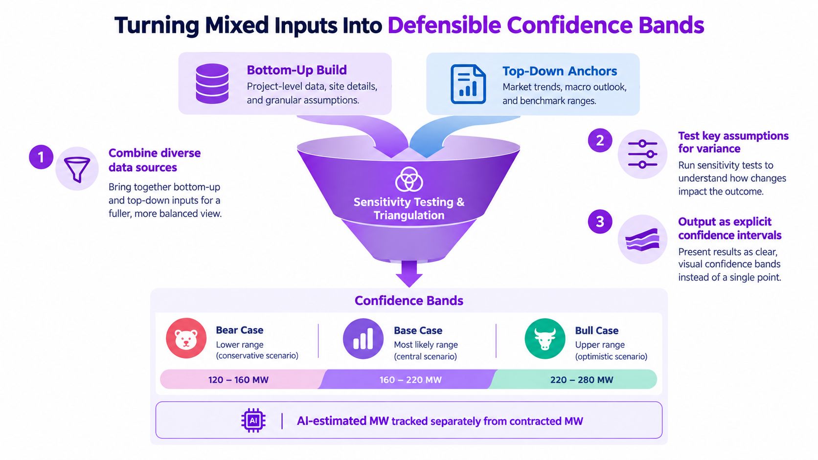
General guidance on market size estimation increasingly emphasizes explicit assumptions, triangulation across independent methods, and ranges rather than single-point claims. It also highlights a practical gap in many market-sizing guides: too few explain how to quantify uncertainty rigorously when data is scarce, even though simulation and uncertainty-aware methods are becoming more relevant in fast-moving sectors uncertainty-aware market size estimation methods.
For data center capacity, the swing factors are usually straightforward:
- Average site MW assumptions: especially where some facilities are estimated rather than disclosed
- Pipeline conversion assumptions: how much planned capacity is treated as likely supply
- Tier mix assumptions: the share of hyperscale, colocation, edge, or enterprise capacity included in scope
A disciplined scenario model flexes only the assumptions that materially move the answer. It does not rebuild every variable at once.
Read divergence as a signal, not an inconvenience
When top-down anchors and bottom-up totals land in a similar range, confidence improves. When they don't, that divergence is useful. It often points to one of three problems: the site universe is incomplete, the pipeline is overstated, or the capacity conversion logic is too aggressive.
That is why low, base, and high cases matter. They force the rationale into the open. A scenario range isn't a hedge against accountability. It's a record of what assumptions are carrying the estimate.
Turning Mixed Inputs Into Defensible Confidence Bands
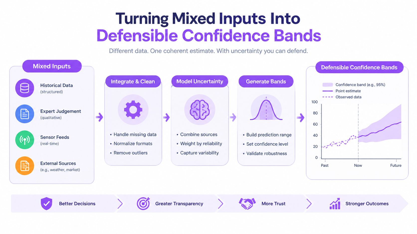
Most weak market estimates fail for the same reason. They combine hard data, soft signals, and inferred values into one total, then present the output as if every row had equal evidentiary weight.
That approach is especially risky in capacity markets because AI-estimated MW and operator-disclosed MW are both useful, but they mean different things. One is a measured or reported claim. The other is an analytical approximation. They should travel through the model in parallel before they meet in the final range.
Separate certainty classes first
A defensible process starts by grouping rows by source quality. One group contains disclosed capacity. Another contains estimated capacity. A third may contain pipeline records with no reliable MW disclosure but enough evidence to support a bounded estimate.
Then assign each row a low and high bound. The width of that bound should reflect factors such as source quality, recency of the evidence, and maturity of the project status. Operational assets with disclosed MW usually deserve narrower bands than planned campuses with inferred power.
Turn the total into a range, not a performance
A confidence band is not a decorative chart around a preferred answer. It is the output of assumptions that have been documented and tested.
A practical regional total usually includes:
- Core estimate: probability-weighted MW based on current evidence
- Lower bound: conservative treatment of estimated and earlier-stage pipeline rows
- Upper bound: more expansive treatment where source quality and stage maturity justify it
- Disclosure note: explicit split between disclosed and estimated contributions
The audience should be able to tell which part of the estimate is solid, which part is conditional, and what would cause the range to widen.
Market size estimation becomes more useful than a static TAM slide. A confidence band tells decision-makers which markets are large, which are merely noisy, and which deserve more diligence before capital or strategy gets attached to them.
Common Pitfalls in Data Center Market Sizing
Bad capacity estimates rarely fail because of arithmetic. They fail because of hidden rule changes inside the model.
The errors that distort the total
One common problem is definitional drift. The estimate starts with one scope, then expands. A model may begin with wholesale-ready capacity and later absorb enterprise facilities or small edge sites without a clear rule change.
Another is pipeline double-counting. A campus appears as planned in one source and under construction in another. If both rows survive the update cycle, the market grows on paper without a single watt being added in reality.
A third problem is confidence laundering. Disclosed MW and estimated MW get blended into one subtotal with no note explaining the split. The output looks authoritative, but the certainty has been overstated.
The last one is unit substitution. Capacity analysis drifts into revenue logic midway through the build. The model stops answering a supply question and starts answering a monetization question without warning the reader.
| Pitfall | Diagnostic Test | Corrective Action |
|---|---|---|
| Definitional drift | Does the inclusion rule stay constant across countries, operators, and status groups? | Lock the market definition before aggregation and document exclusions |
| Pipeline double-counting | Can one project appear in more than one stage at the same time? | Timestamp status changes and retire superseded rows |
| Blended certainty | Can the output separate disclosed MW from estimated MW? | Maintain separate columns and footnote the split in every summary table |
| Unit substitution | Did the model switch from MW to revenue or site count without a formal bridge? | Keep one primary unit and relegate secondary units to supplemental views |
| Hidden scope creep | Did small facilities or non-target facility types enter the SAM inconsistently? | Apply one threshold rule and test every row against it |
The audit questions worth asking early
A disciplined analyst asks uncomfortable questions before the investment committee does:
- Scope test: Is every included facility type part of the stated market?
- Status test: Has each project been assigned one current stage only?
- Unit test: Is the primary output still MW, not an accidental blend of metrics?
- Confidence test: Can every summary table show what is disclosed versus inferred?
Those checks don't slow the model down. They stop it from becoming unpublishable later.
A Practical Playbook for Your Next Estimate
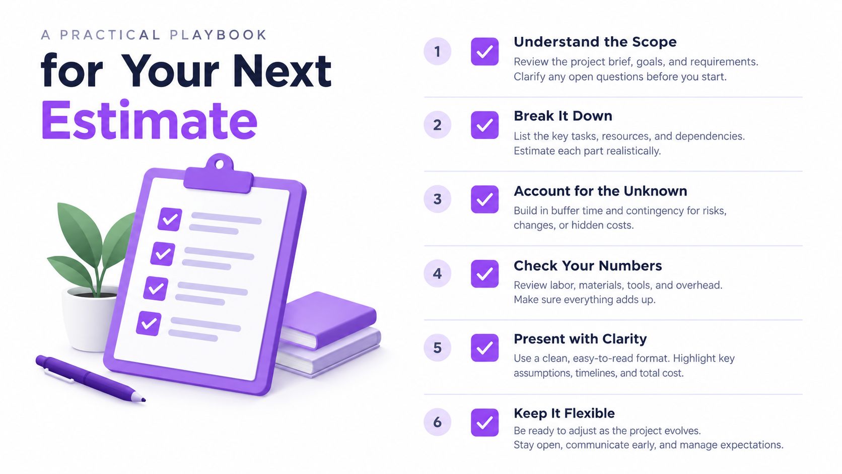
A usable estimate doesn't begin with the number. It begins with the rulebook. That rulebook should fit on one page.
The six-step workflow
- Define the scope clearly. Decide the geography, facility types, customer segment, and pipeline stages that belong in the estimate.
- Choose the primary unit. For capacity markets, that usually means IT load in MW. Keep revenue, site count, or hall count as secondary outputs.
- Build the row-level inventory. Classify each facility once by operator, market, and current status.
- Separate disclosed and estimated values. Never merge them without preserving the split.
- Layer top-down anchors and scenarios. Use low, base, and high cases to test the assumptions that move the result most.
- Publish the range with limits. Document what the model includes, what it excludes, and what would change the confidence band.
The short checklist that catches most problems
- Unit consistency: every subtotal rolls up in the same unit
- Source dating: each row reflects the latest known status
- Confidence labeling: disclosed and AI-estimated MW remain distinct
- Scenario logic: each range has explicit assumptions behind it
- Limits paragraph: the final output states where evidence is strong and where it is conditional
The last item is the one many teams skip. They shouldn't. Market size estimation becomes more persuasive when it admits its limits plainly. Pipeline attrition, uneven disclosure, and geographic granularity are not embarrassing caveats. They are part of the result.
A market estimate survives scrutiny when another analyst can inspect the assumptions, rebuild the logic, and understand why the number lands where it does.
Data Centers List offers a structured way to work from facility-level evidence rather than abstract TAM rhetoric, including operational, planned, and under-construction sites with disclosed and AI-estimated IT power fields kept distinct. For analysts sizing capacity markets, that makes it easier to build MW-grounded inventories, test pipeline assumptions, and present confidence bands that can survive review. Explore the dataset and market views at Data Centers List.