How Much Power Does a Data Center Use: 2026 Guide
Discover how much power does a data center use from small edge sites to hyperscale campuses, with IT load, PUE, and real MW examples.
16 min read
A typical single data center draws between 1 MW and 100 MW at the facility level, while hyperscale campuses can reach 200 MW to over 1 GW. The IT load inside is roughly 60% to 85% of that total once PUE is accounted for.
That range sounds broad because “data center” can mean a room with a few racks, a colocation building, or a multi-building campus connected to a major grid. The most important distinction is between IT load, the electricity consumed by servers, storage, and networking, and total facility draw, the power entering the site after cooling, distribution, and other support systems are included.
At the global level, the scale is already material. Data centers used about 415 TWh of electricity in 2024, around 1.5% of world electricity consumption, according to the International Energy Agency's analysis of energy demand from AI. The IEA says demand grew by about 12% annually over the previous five years and could roughly double to 945 TWh by 2030, approaching 3% of global electricity use. Those totals are facility-level electricity figures, not merely processor consumption.
Table of Contents
- The Power Range From a Single Rack to a Hyperscale Campus
- What Drives a Data Center's Electricity Bill
- Understanding PUE and Why Two Sites With the Same IT Load Draw Different Power
- Typical Power Use by Facility Type From Edge to Hyperscale
- Real Disclosed and Estimated MW Figures From Major Markets
- How to Estimate a Data Center's Power Use in Megawatts
- What to Look at First When You Ask How Much Power a Site Uses
The Power Range From a Single Rack to a Hyperscale Campus
The cleanest way to answer how much power a data center uses is to move from the smallest useful unit, the rack, to the largest operating unit, the campus. A standard rack may require only a few kilowatts, while a hyperscale site can draw hundreds of megawatts or more from the grid.
The figures below are analytical planning ranges, not universal benchmarks. They show the order of magnitude for different facility scales. The IT figures describe computing equipment. The facility figures include the supporting infrastructure required to keep that equipment powered and within operating conditions.
| Facility Scale | Typical IT Load | Total Facility Draw |
|---|---|---|
| Single 42U rack | 5 to 15 kW | Higher than IT load after facility overhead |
| Small enterprise or edge room | 0.5 to 2 MW | Above 0.5 to 2 MW |
| Typical colocation hall | 5 to 30 MW | Above 5 to 30 MW |
| Hyperscale campus | 200 MW to over 1 GW | 200 MW to over 1 GW |
A rack's demand depends on the equipment installed, its utilization, and the workload mix. General-purpose enterprise computing tends to occupy a lower density band. High-density accelerated computing pushes rack demand upward, and that increase affects not only the servers but also the cooling architecture and power distribution design.
Why the meter matters
A site advertised as having a 10 MW IT capacity won't necessarily draw 10 MW at the utility meter. The meter sees the IT load plus cooling, power conversion losses, pumps, fans, lighting, controls, and other facility systems. The relationship is expressed through Power Usage Effectiveness, or PUE.
A useful mental model is simple:
- IT load: Servers, storage, and network equipment.
- Facility overhead: Cooling, electrical distribution, lighting, security, and controls.
- Grid draw: IT load multiplied by PUE.
The global figure of 415 TWh in 2024 matters because it prevents facility-level examples from being viewed in isolation. The IEA's global assessment places individual campuses inside a rapidly expanding electricity system, where local projects can affect substations, transmission planning, and community discussions even when each facility represents only part of regional demand.
What Drives a Data Center's Electricity Bill
A facility's utility bill reflects more than its servers. IT load supplies the computing work, while cooling, electrical distribution, and building systems determine the additional power required at the meter. The four categories are useful for separating verified computing capacity from total facility draw.
The split varies with climate, building design, equipment age, rack density, and operating conditions. PUE, or Power Usage Effectiveness, measures total facility energy divided by IT equipment energy. That definition lets analysts compare sites even when operators do not disclose every subload.
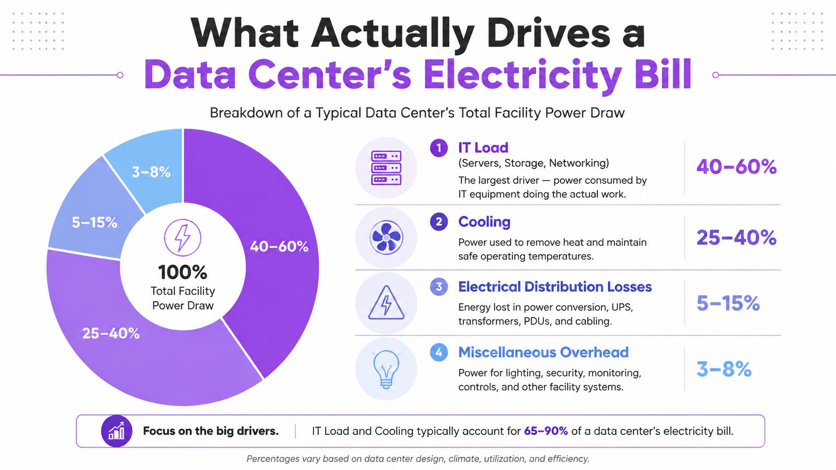
The four components behind total draw
IT load includes servers, storage, and network equipment. It rises with the number of active machines, processor type, storage activity, network traffic, and workload utilization. A site may advertise substantial installed IT capacity while drawing far less if racks await deployment or systems run below full utilization.
Cooling removes heat from IT equipment and maintains acceptable temperature and humidity conditions. Air handlers, chillers, cooling towers, pumps, fans, and liquid-cooling loops all consume electricity. Local weather, heat-rejection equipment, indoor set points, and rack density shape this demand. Higher-density accelerated computing can therefore increase facility draw through both the computing load and the cooling system supporting it.
Electrical distribution losses occur as power passes through transformers, switchgear, uninterruptible power systems, power distribution units, and cabling. Efficient designs reduce conversion losses, while redundancy and resilience requirements can add equipment and power-conversion stages.
Miscellaneous overhead includes lighting, security, monitoring, building controls, fire protection, and other services. These loads are usually smaller than IT and cooling, but they remain part of the utility-meter reading.
Why operators control only part of the result
Tenants can influence their server fleet, storage architecture, utilization, and rack density. Operators and building owners control cooling topology, electrical design, maintenance, and control systems. Climate also constrains the available heat-rejection strategy.
Practical rule: Label every capacity figure as either IT load or total facility draw before comparing sites.
The original benchmark dataset reported an average PUE of 1.83, showing why identical IT megawatts can produce different utility requirements. A lower-PUE facility sends a larger share of grid intake to computing. A higher-PUE facility assigns more of its draw to support infrastructure, even when the server workload is identical. For market analysis, disclosed IT MW should therefore remain separate from any modeled estimate of total site draw.
Understanding PUE and Why Two Sites With the Same IT Load Draw Different Power
PUE is a ratio, not a direct measure of server efficiency. It divides total facility power by IT equipment power. A theoretical PUE of 1.0 would mean every unit entering the building reaches IT equipment, with no cooling or other overhead. Normal operations cannot reach that condition.
The calculation is:
Total facility draw = IT load × PUE
A site with a 50 MW IT load and a PUE of 1.2 draws 60 MW from the grid. At a PUE of 1.8, the same IT load produces 90 MW of facility demand. The 30 MW difference comes from cooling, electrical distribution, and other support systems, not from additional computing.
| PUE | Total Grid Draw | Cooling + Overhead Share | Typical Site Profile |
|---|---|---|---|
| 1.2 | 60 MW | 10 MW | Highly optimized design |
| 1.3 | 65 MW | 15 MW | Efficient modern facility |
| 1.8 | 90 MW | 40 MW | Older or less optimized site |
Why PUE changes from site to site
Climate affects the support load. A facility in a cool environment may reject heat with less mechanical cooling during suitable conditions, while a hot environment may require more active cooling and heat rejection. The design also matters. Air cooling, direct liquid cooling, and immersion cooling place different demands on pumps, heat exchangers, chillers, airflow, and electrical distribution.
Compute density changes the comparison as well. A lightly loaded enterprise room may use conventional cooling, while a high-density accelerated-computing hall may require liquid cooling and a different power architecture. Analysts should therefore read PUE alongside the workload and operating condition that produced it.
As noted earlier, the LBNL dataset reports an average PUE of 1.83. That figure should not be treated as a current universal average for every market. Its analytical value is narrower: it shows why disclosed IT capacity cannot, by itself, establish grid impact. The Lawrence Berkeley benchmarking guide provides the underlying framework for interpreting the ratio.
The distinction matters when comparing verified disclosures with modeled capacity. A published IT MW figure identifies computing capacity or consumption only if its scope says so. An AI-estimated capacity figure can support a market model, but converting either figure into total facility draw requires an explicit PUE assumption.
A facility profile such as the Syracuse University Green Data Center should therefore be read by scope. Determine whether the stated power represents installed IT capacity, measured IT consumption, contracted utility capacity, or total facility demand before using it in a comparison.
Typical Power Use by Facility Type From Edge to Hyperscale
An edge micro-site and a hyperscale campus may support similar cloud workloads, but their power profiles diverge sharply. The difference appears in both IT load, the electricity used by computing equipment, and total facility draw, which also includes cooling, power delivery, and other site systems.
The table below applies a planning PUE of 1.3 to show how an assumed IT load translates into estimated facility draw. These are directional bands, not measured values for every facility. A disclosed figure should be labeled separately from an AI-estimated capacity or a planning assumption.
| Facility Type | Typical IT Load (MW) | Total Facility Draw at PUE 1.3 (MW) | Typical Scale | Workload Profile |
|---|---|---|---|---|
| Edge micro-site | Below 1 | Below 1.3 | Small rack group or modular room | Latency-sensitive services, local processing |
| Enterprise room | 0.5 to 5 | 0.65 to 6.5 | Dedicated room or small building area | Corporate applications, storage, private systems |
| Colocation building | 5 to 50 | 6.5 to 65 | Multiple halls and customer suites | Mixed tenants, cloud access, network interconnection |
| Hyperscale campus | 50 MW hall, 200 MW to over 1 GW campus | 65 MW hall, 260 MW to over 1.3 GW campus | Multi-building campus | Cloud platforms, large-scale analytics, accelerated computing |
Edge and enterprise footprints
Edge facilities keep their individual IT load small by placing processing near users, devices, industrial systems, or communications networks. Their total facility draw remains higher than the IT figure because each site still requires power conversion, cooling, and monitoring. Operators may deploy many sites across separate locations, so a single-site profile can understate the combined footprint.
Enterprise rooms generally have steadier workloads than hyperscale campuses. Demand can rise as organizations add applications, storage, and internal services. Analysts should distinguish installed rack capacity from equipment that is running, then apply the relevant PUE assumption to estimate total facility draw.
Colocation and hyperscale campuses
Colocation halls combine several customers, so building-level facility draw reflects unrelated workload profiles. A customer may reserve IT capacity without using it fully. Contracted capacity, commissioned capacity, measured IT load, and utility draw therefore describe different operating conditions.
Hyperscale campuses sit at the upper end because they combine large server populations with extensive electrical and cooling infrastructure. Accelerated computing can raise rack density and increase the supporting facility draw, particularly where specialized thermal systems are required.
A named profile still needs a scope check. The EdgeConneX Toronto facility profile should be read according to whether its figure represents IT capacity, total facility demand, or another capacity label. That distinction determines whether it can be compared directly with the table's modeled IT and facility bands.
The market pattern is clear. Edge nodes use relatively little power individually but multiply across locations. Hyperscale campuses concentrate much larger facility draws in fewer grid connections, while scale can improve the relationship between computing output and supporting overhead.
Real Disclosed and Estimated MW Figures From Major Markets
Named markets show why verified disclosure and modeled capacity must remain separate. Public records may report a utility connection, campus plan, or operator capacity. A directory may instead estimate IT power from facility attributes when no direct figure is available. The first set describes what was disclosed. The second describes an analytical assumption. Neither should be treated as measured consumption without meter data.
In 2024, the United States accounted for 45% of global data center electricity consumption, China for 25%, and Europe for 15%, according to the IEA executive summary on energy and AI. This concentration places a small group of power markets at the center of grid planning. These regional shares describe electricity consumption, not necessarily installed IT load or a single site's facility draw.
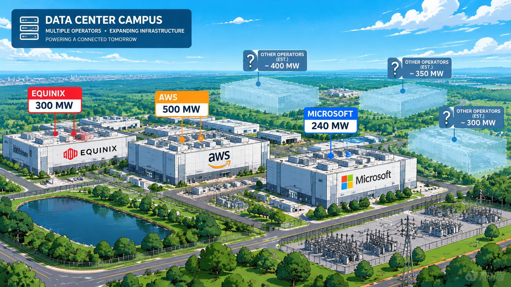
How to read market-level figures
A Northern Virginia campus described in the hundreds of megawatts should be read as a facility-level or interconnection figure unless the disclosure identifies IT load. An Ireland cluster approaching 1 GW combined is a market or cluster total, not automatically the demand of one building. The aggregation boundary can matter as much as the MW value.
A Nordic site may achieve lower overhead through its climate and heat-rejection design. That does not make its total facility draw lower than another site with the same IT load unless both PUE values and operating conditions are calculated. Singapore offers a different constraint, with facility expansion limited around 60 MW. There, available grid capacity affects site selection before operating efficiency becomes the deciding factor.
Secondary-market colocation sites sit below these regional anchors. Their smaller facilities may support enterprise workloads, network interconnection, or local cloud demand. A profile such as Google's Elmina Business Park data center is useful only when its location, operator, status, figure type, and date are recorded together. A disclosed facility MW value and a directory's modeled IT MW should appear as separate fields, with the assumed PUE shown before converting IT load into total facility draw.
Evidence rule: A disclosed MW figure records what an operator, utility, or planning document stated. An estimated MW figure records a model assumption. Neither represents measured consumption without meter data.
AI expansion makes old figures harder to interpret. The IEA's key questions on energy and AI reports that AI-focused data-center electricity use surged 50% in 2025 and projects global data-center demand to rise from 485 TWh in 2025 to 950 TWh by 2030, around 3% of global demand. It also identifies 195 TWh for cooling and other infrastructure in 2026, up from 159 TWh in 2025, while AI-optimized servers account for 31% of data-center electricity consumption. The implication is twofold. AI raises IT demand, while cooling, other infrastructure, and unused capacity determine how much additional power reaches the facility meter.
How to Estimate a Data Center's Power Use in Megawatts
A defensible estimate separates IT load from the electricity drawn by the whole facility. Start with rack count and workload density:
Rack count × average kW per rack ÷ 1,000 = IT load in MW
Then convert the IT figure into an estimated meter-side requirement:
IT load in MW × assumed PUE = total facility draw in MW
As defined in section 1, PUE equals total facility energy divided by IT equipment energy. The ratio should be applied only after establishing the IT load and confirming its scope.
Rack density must reflect the equipment mix. A planning model can test 8 kW, 15 kW, 30 kW, or 60+ kW per rack, but these are scenario assumptions, not universal averages. Conventional enterprise equipment generally fits the lower scenarios, while high-density accelerated computing belongs toward the upper end. A directory's modeled IT MW should therefore show the rack count, density assumption, and PUE separately from any disclosed facility MW figure.
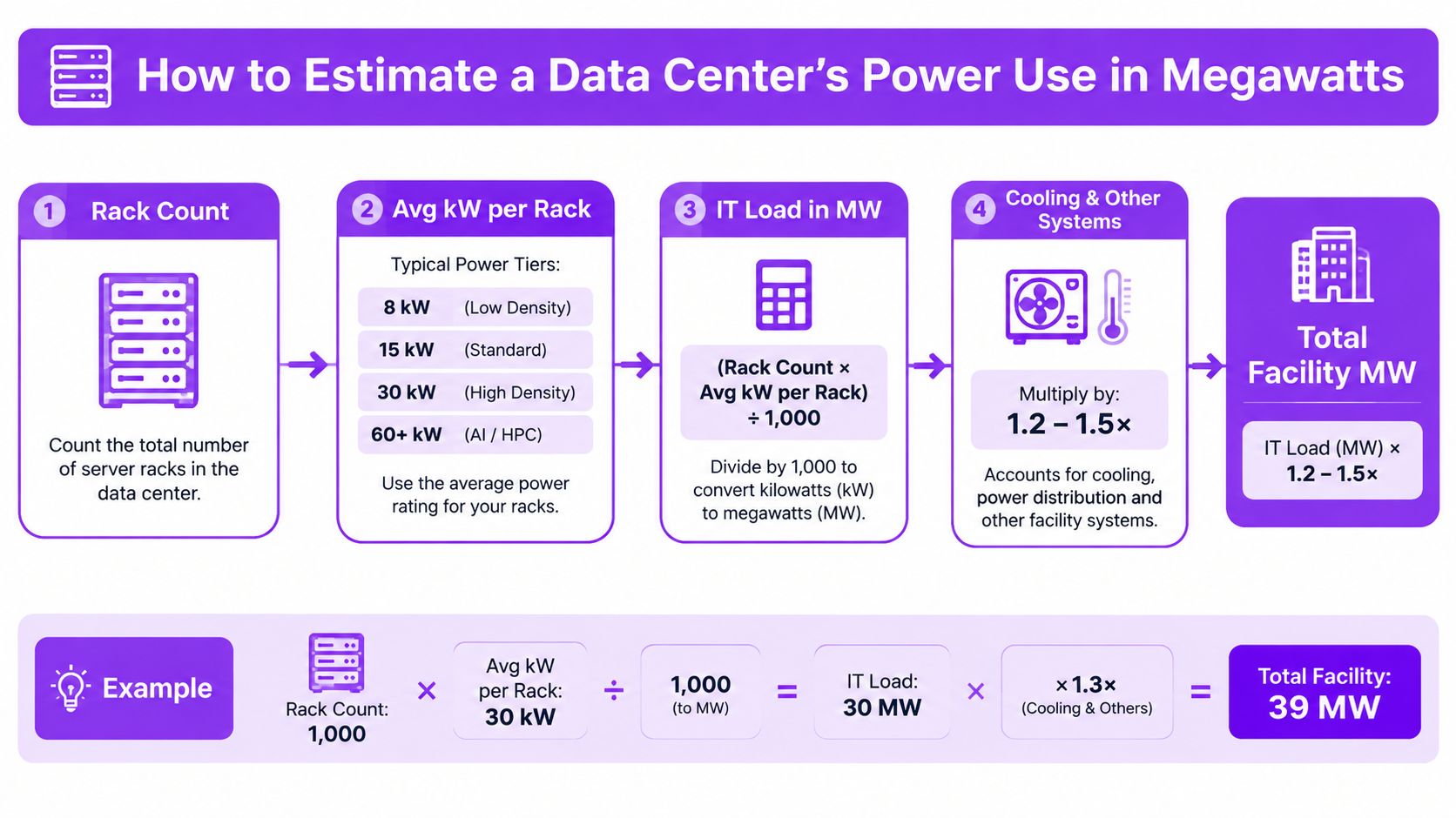
A worked planning example
For 200 racks averaging 15 kW, the calculation is:
- 200 × 15 kW = 3,000 kW
- 3,000 kW ÷ 1,000 = 3 MW IT load
- 3 MW × 1.3 PUE = 3.9 MW total facility draw
The resulting 3.9 MW is an estimated demand at the facility meter under the stated assumptions. It does not establish continuous consumption or measured energy use.
Utilization changes the operating estimate. A researcher can model 50% to 80% utilization and apply that adjustment to the IT portion before adding facility overhead. Redundancy requires a separate field. N+1 or 2N designs can increase installed equipment and electrical capacity, while nameplate redundancy does not equal simultaneous operating load.
Inputs needed for a credible estimate
- Rack inventory: Separate occupied, reserved, and empty rack positions.
- Density profile: Assign different kW assumptions to enterprise, storage, network, and accelerated-computing racks.
- Utilization: Separate commissioned capacity from measured operating demand.
- PUE scope: Confirm whether the ratio covers the entire facility or a defined building or system boundary.
- Expansion phase: Identify current operations, fit-out capacity, or a future build.
- Redundancy design: Record N+1, 2N, and uncommissioned reserve capacity separately.
The estimate is useful only when its inputs remain visible. A round-number figure without rack count, PUE scope, date, or facility status is a screening estimate, not an operating fact.
What to Look at First When You Ask How Much Power a Site Uses
The answer should begin at the utility meter. Total facility draw is the only figure that directly answers how much electricity a site takes from the grid at a given moment or over a stated period. IT load alone can overstate current consumption when equipment is planned but not installed, or understate grid impact when cooling and distribution overhead are substantial.
A fast diagnostic sequence has four checkpoints.
Total facility draw at the meter. Utility bills, interval data, or interconnection records provide the strongest evidence of grid impact. The time period matters because instantaneous demand, peak demand, and annual energy answer different questions.
Committed IT load versus actual IT load. A site may have contracted capacity, installed capacity, and active equipment capacity at the same time. Those labels shouldn't be treated as interchangeable.
Cooling topology and current use. Air systems, liquid systems, chillers, pumps, fans, and heat-rejection equipment can produce very different overhead profiles. A capacity figure for cooling equipment doesn't prove that the equipment is operating at full load.
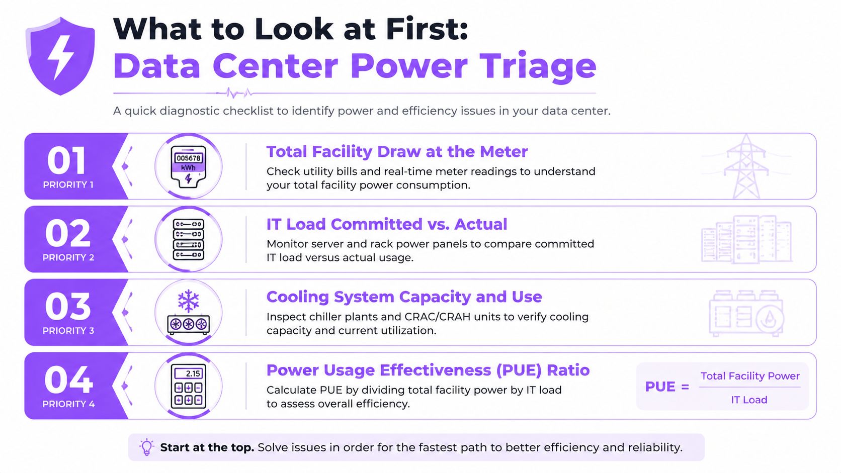
- The latest PUE with defined boundaries. A PUE value is meaningful only when the numerator, denominator, date, and reporting boundary are clear. The LBNL benchmarking guide provides the formal definition needed to check that scope.
Red flags in public power data
Round-number MW claims often indicate a planning estimate rather than measured consumption. Missing utility interconnection evidence, an old publication date, and a PUE value without scope boundaries create the same problem. The IEA's regional figures show why local validation matters, since the United States, China, and Europe together represented the overwhelming majority of global data-center electricity consumption in 2024, with the exact regional shares documented in the IEA executive summary.
Decision rule: Use meter draw for grid impact, IT load for computing capacity, PUE for efficiency, and annual energy for carbon accounting.
Data Centers List provides facility profiles and market views that distinguish disclosed capacity from AI-estimated capacity, helping researchers compare sites without treating modeled figures as measured consumption. Visit Data Centers List to examine facility status, operator information, IT power fields, and market-level capacity in one directory. For any serious assessment, pair the directory figure with the latest operator, utility, or planning disclosure before making a grid, investment, or development decision.